
Autoresearch Journey Figures
A self-contained package for the autoresearch writeup figures, including rendered plots, raw run data, portable plotting scripts, and the code snippets behind each labeled rung.
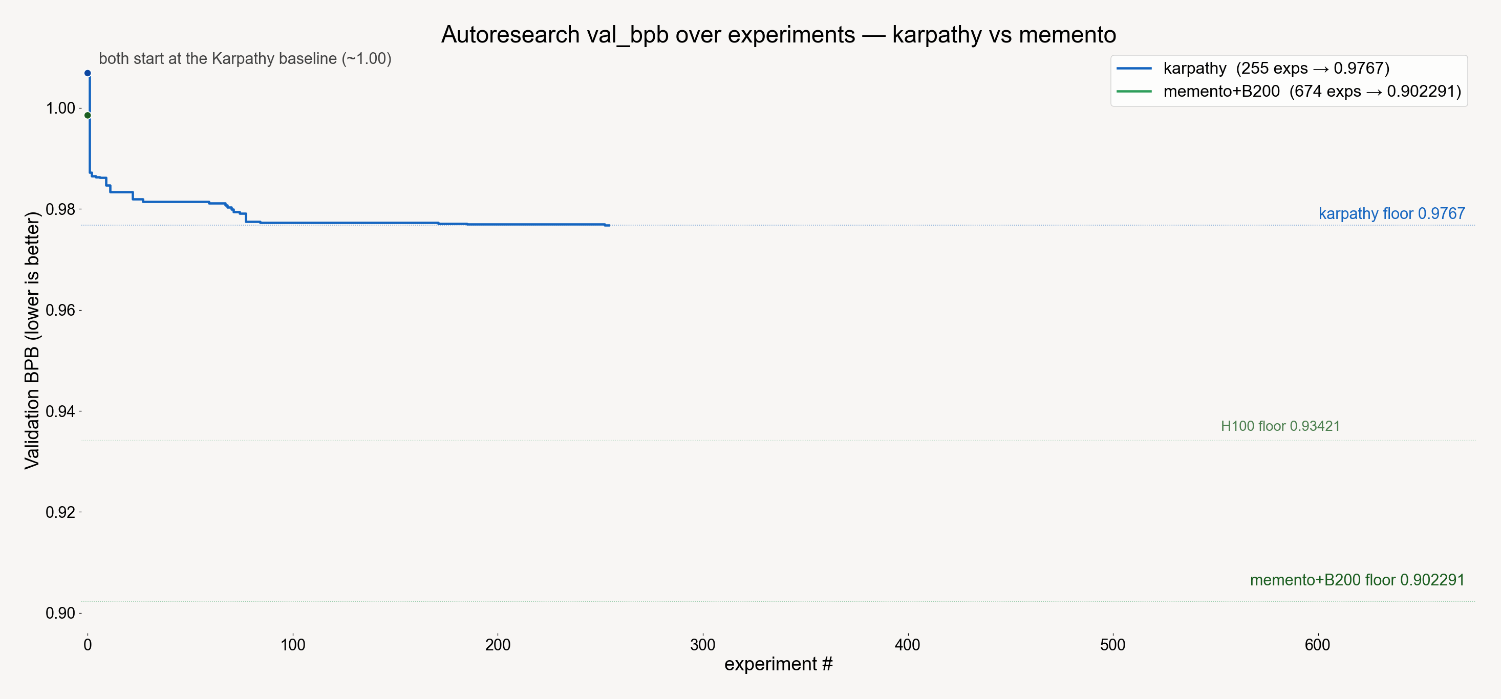
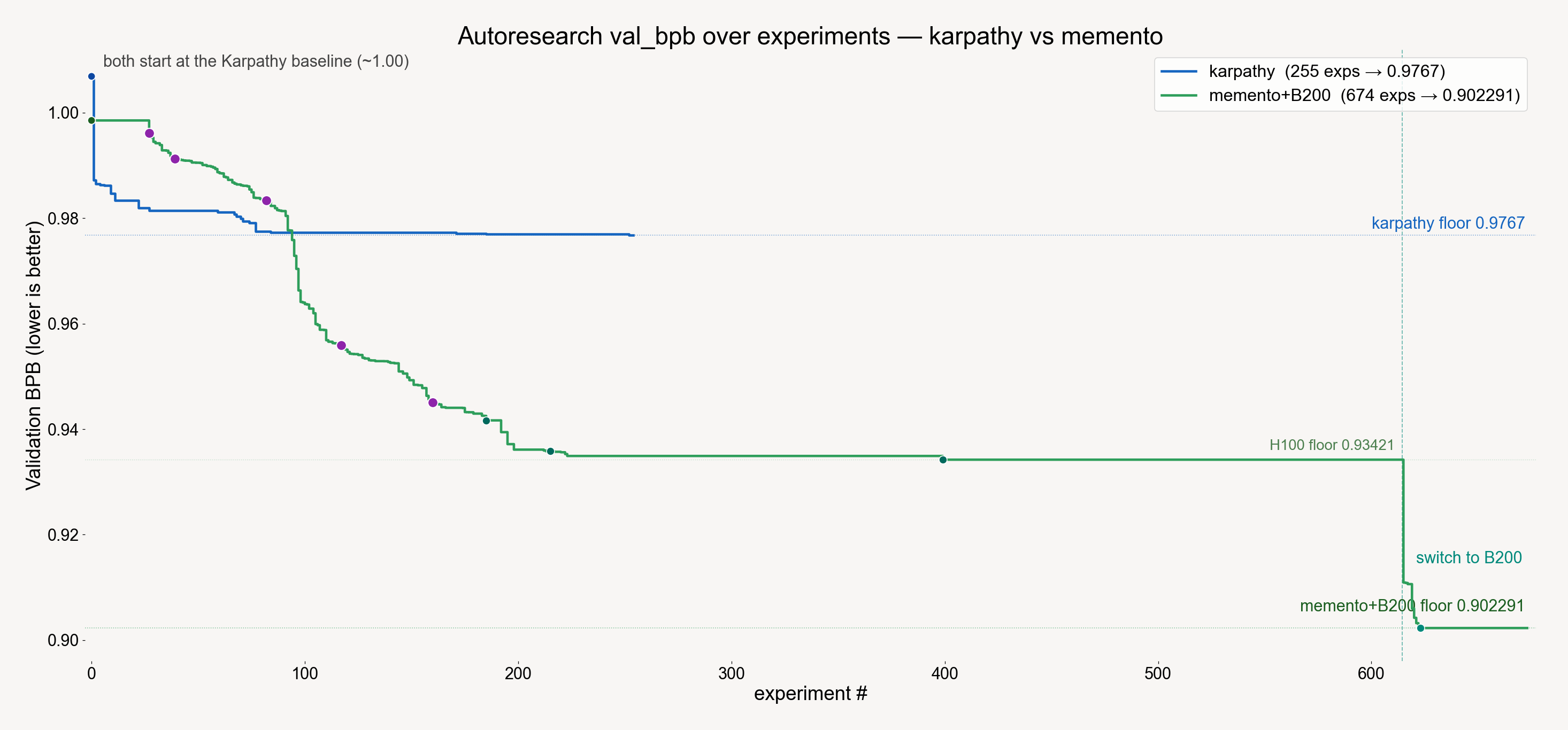
Baseline
Only the baseline trajectory is visible.
- ① Karpathy seed 0.9961
- ② + Muon optimizer 0.9913
- ③ + value embeddings 0.9834
- ④ + n-gram memory memory ≠ compute · 0.9559
- ⑤ + window + softcap recursive 0.9442 · H100 path 0.9451
- ⑥ throughput retune max-autotune + ngram 64→48
- ⑦ width search compute-optimal dim 768→640
- ⑧ H100 joint BO 0.93421
- ⑨ B200 tuning 0.902291
One curve, nine rungs: 0.9961 → 0.93421 (H100) → 0.902291 (B200)
TL;DR. Under a token-bound budget (one GPU, a fixed 300s of training, minimize val_bpb), the agent walked down a single descending curve in two moves — first discover the right architecture by judgment (rungs ①–⑤), then squeeze it dry with Bayesian optimization (rungs ⑥–⑧) — taking the Karpathy seed (0.9961) to 0.93421 on H100, then continuing the same recipe on a B200 (⑨) to 0.902291, about 0.024 below the current #1 (forge, 0.9264). Retraced below, rung by rung, as what the agent was thinking → what it did → what it measured → how it updated.
Why the problem is hard, and what the real objective is
The rules are simple: one GPU, training time fixed at 300 seconds, lower val_bpb is better. It's token-bound — at ~40% MFU in 300s the model sees only ~190M tokens. So the objective is really a product of two axes:
val_bpb↓ ⇔ max(tokens seen × loss-drop per token)
Tokens are the binding constraint (the dominant axis), but "make each token count more" is just as much a goal. Every rung below maps onto one of these two axes.
Discover — find the architecture by judgment (rungs ①–⑤)
Five rungs, big jumps, judgment-driven. By rung ⑤ the recipe already matches recursive's official recipe — and most of the total drop is already done.
① Karpathy seed — 0.9961
The plain decoder-LM baseline. This is where the memento run starts, from the same baseline family as the Karpathy-style tuning it's racing. Everything below is added on top of this.
② + Muon optimizer — 0.9913
Belief: I don't know the terrain. Don't reach for more depth/width first — under a token-bound budget more parameters just cost throughput. Reach for a better optimizer: spend the cheap win on the efficiency axis.
Measured: Swapping AdamW → Muon (Nesterov momentum + Polar-Express orthogonalization of the gradient) gives the first clear drop, and the largest single step of the whole run.
Updated: The bottleneck isn't capacity, it's how much each token's gradient is worth. Make every token count more.
③ + value embeddings — 0.9834
A cheap gated per-token embedding injected straight into the attention value stream — more signal per token at almost no throughput cost. → 0.9834.
④ + n-gram memory — 0.9559 (the "memory ≠ compute" pivot)
Belief: Tokens are expensive; memory and parameters are cheap. Much of web-text predictability is local n-gram statistics — why make a transformer spend precious tokens learning these slowly by gradient descent? Just memorize them in a hash table.
Measured: Hashed bigram/trigram tables added to the value stream → 0.9559, the single biggest architectural jump.
Updated: The real lever is switching to a "memory axis," not piling onto the compute axis. n-gram is special: ~0 FLOPs and it frees the precious tokens for the hard parts.
⑤ + window + softcap — 0.9451 (= recursive 0.9442)
Patterned attention windows (tiny/short/long, last layer full) make attention cheaper → more tokens/sec; a tanh logit softcap stabilizes the softmax so a higher LR is safe. → 0.9451, which already ties recursive's official recipe.
Discover takeaway: architecture discovery is prior/judgment-driven — few steps, big jumps. At 0.9451 the curve already matches recursive.
Squeeze — press it to the noise floor with BO (rungs ⑥–⑧)
With the architecture fixed, the rest is squeezing the continuous hyperparameter space. The absolute drop here is small (0.9451 → 0.93421, ~−0.011) but it took 400+ evaluations — the "last mile."
Belief: The architecture is right; now drive the continuous knobs (size, LR, schedule) to their limit with Bayesian optimization — a from-scratch numpy GP + Expected-Improvement.
One detail worth naming, because it's really the loop: this is discovery at two grains at once. BO sweeps the continuous knobs; alongside it, the agent sets which knobs are worth sweeping and how far, then reads the BO log and, when progress stalls, redraws that box by reflection. Rungs ⑥–⑨ are exactly that — each is another move in the same discovery, made after seeing where the last one got stuck.
⑥ throughput retune — max-autotune + ngram 64→48
The throughput axis: torch.compile max-autotune plus trimming the n-gram table multiplier 64→48 buys tokens/sec with no loss of quality.
⑦ width search — compute-optimal dim 768 → 640
The counterintuitive "go narrow": BO pushes "capacity isn't the bottleneck" to its conclusion — a narrower model (dim 768 → 640) eats more tokens/sec, and under a fixed budget more data beats more parameters.
⑧ H100 joint BO — 0.93421
Joint GP-EI over all the continuous knobs (size, LR, schedule, momentum) → 0.93421.
Updated (knowing when to stop): After 400+ evals, single-run improvement < 0.0002 — smaller than seed noise. I can no longer tell signal from luck. That's the noise floor. Stop.
Squeeze takeaway: the BO squeeze is data/search-driven — hundreds of steps, small wins. On the same H100 the curve now sits below recursive (0.9442).
B200 — the same recipe, more tokens (rung ⑨)
Belief: Is 0.93421 a recipe ceiling or a hardware ceiling? The #1, forge, is 0.9264 on a B200, which fits ~2.4–2.7× the tokens of an H100 in 5 min. This is a throughput problem, so the gap is probably hardware.
First, a make-or-break dependency — FA4. The B200's edge rides almost entirely on FlashAttention-4: FA3 is Hopper-only, so on a B200 without FA4 the tensor cores idle and a B200 can be worse than an H100. Our recipe already ships the same FA4 CUTLASS custom-op, so it kicks in automatically on Blackwell.
⑨ B200 tuning — 0.902291
Port the H100 champion as-is → 0.9109, already below both forge (0.9264) and overmind (0.9274). Then the same squeeze, with the H100 principles flipped by the larger token budget — "go narrow" becomes "go moderately wider": here the agent redraws the box in the opposite direction once the B200 log says so —
- compute-optimal width moves wider: dim 768 (0.902) > dim 640 (0.911);
- don't add depth: depth 10 (0.906) is worse than depth 8 (0.902);
- widen n-gram capacity (48→64) — the core edge over forge;
- BO presses matrix_lr down to 0.035.
Result: 0.902291, ~0.024 below the #1.
| recipe | val_bpb |
|---|---|
| ours (B200) | 0.902291 |
| forge #1 (B200) | 0.926381 |
| overmind #2 (B200) | 0.927396 |
Three counterintuitive conclusions
| intuition | what the agent revised after measuring |
|---|---|
| if it's not good enough, make it bigger | capacity cliff — under a token-bound budget, bigger is a net loss |
| pile on compute / parameters | memory ≠ compute — spend the cheap resource: sparse hashed memory (rung ④) |
| bigger models are better | go narrow when you should (H100 768→640), wider when you should (B200) — it's all about seeing more tokens |
It's all discovery — two methods, one loop
It doesn't really matter which rung was a judgment call and which was BO — and that's the point. Both are discovery, just at different grains:
- a prior-driven discovery of what to build and where to look — the agent (LLM ⊗ human ⊗ web) proposes techniques, draws the box of knobs worth tuning, and reflects on the log to redraw it;
- a Bayesian discovery of the exact settings — a surrogate + Expected-Improvement presses that box to the noise floor.
They're the same activity at two resolutions, taking turns in one loop until the curve flattens: discover the structure, discover the settings, read the result, discover again. The discover→squeeze arc — and the B200 re-run — is just this one loop playing out.
Included
Journey Rungs
- Karpathy seed: the plain decoder LM baseline at 0.9961 val_bpb.
- Muon optimizer: Nesterov momentum plus Polar-Express orthogonalization.
- Value embeddings: gated per-token embeddings injected into the value stream.
- N-gram memory: bigram and trigram statistics hashed into large lookup tables.
- Sliding window: patterned tiny, short, and long attention windows.
- Softcap: tanh-capped logits to stabilize the output distribution.
- Modern arch: QK norm before rotary and ReLU squared MLP activation.
- Width search: compute-optimal dim 640 found by Bayesian optimization.
- Joint BO: numpy GP plus expected improvement reaching 0.93421.
- B200 tuning: the B200 continuation reaches 0.902291 val_bpb.
Resources
Package README
Layout, regeneration commands, and the high-level file map.
Bundle map
Figure to script to data mapping, plus provenance notes.
Code snippets
Verbatim code anchors for each labeled rung in the journey plot.